TRANSPORT

This keyword data block is used to simulate 1D transport processes that include advection and dispersion, diffusion, and diffusion into stagnant zones adjacent to the 1D flow system. All chemical processes modeled by PHREEQC, including kinetically controlled reactions, may be included in an advective-dispersive transport simulation. Purely advective transport plus reactions--without diffusion, dispersion, or stagnant zones--can be simulated with the ADVECTION data block.

Explanation

Line 0: TRANSPORT

TRANSPORT is the keyword for the data block. No other data are input on the keyword line.

Line 1: -cells cells

-cells--Indicates that the number of cells in the 1D column will be given. Optionally, cells or -c[ ells].

cells --Number of cells in a 1D column to be used in the advective-dispersive transport simulation. Default is 0.

Line 2: -shifts shifts

-shifts--Indicates that the number of shifts or diffusion periods in the advective-dispersive transport simulation will be given. Optionally, shifts or -s[ hifts].

shifts --For advective-dispersive transport, shifts is the number of advective shifts or time steps, which is the number of times the solution in each cell will be shifted to the next higher or lower numbered cell; the total time simulated is . For purely diffusive transport, shifts is the number of diffusion periods that are simulated; the total diffusion time is . Default is 1.

Line 3: -time_step time step

-time_step--Defines time step associated with each advective shift or diffusion period. The number of shifts or diffusion periods is given by -shifts. Optionally, timest, -t[ imest], time_step, or -t[ ime_step].

time step --Time, in seconds, associated with each shift or diffusion period. Default is 0.

Line 4: -flow_direction ( forward, back, or diffusion_only)

-flow_direction--Defines direction of flow. Optionally, direction, flow, flow_direction, -dir[ ection], or -f[ low_direction].

forward, back, or diffusion_only--(1) Forward, advective flow direction is forward; optionally, f[ orward], (2) Backward, advective flow direction is backward; optionally b[ ackward], or (3) Diffusion_only, only diffusion occurs, there is no advective flow; optionally d[ iffusion_only] or n[ o_flow]. Default is forward.

Line 5: -boundary_conditions first, last

-boundary_conditions--Defines boundary conditions for the first and last cell. Optionally, bc, bcond, -b[ cond], boundary_condition, -b[ oundary_condition]. Three types of boundary conditions are allowed at either end of the column (indicated by ):

constant--Concentration is constant 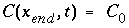, also known as first type or Dirichlet boundary condition. Optionally, co[ nstant] or 1.

closed--No flux at boundary, 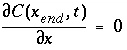, also known as second type or Neumann boundary condition. Optionally, cl[ osed] or 2.

flux--Flux boundary condition, 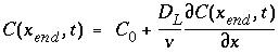, also known as third type or Cauchy boundary condition. Optionally, f[ lux] or 3.

first --Boundary condition at the first cell, constant, closed, or flux. Default is flux.

last --Boundary condition at the last cell, constant, closed, or flux. Default is flux.

Line 6: -lengths list of lengths

-lengths--Defines length of each cell for advective-dispersive transport simulations (m). Optionally, length, lengths, or -l[ engths].

list of lengths --Length of each cell (m). Any number of lengths up to the total number of cells ( cells ) may be entered. If cells is greater than the number of lengths entered, the final value read will be used for the remaining cells. Multiple lines may be used. Repeat factors can be used to input multiple data with the same value; in the example data block, 4*1.0 is interpreted as 4 values of 1.0. Default is 1.

Line 7: -dispersivities list of dispersivities

-dispersivities--Defines dispersivity of each cell for advective-dispersive transport simulations (m). Optionally, disp, dispersivity, dispersivities, -dis[ persivity], or -dis[ persivities].

list of dispersivities --Dispersivity assigned to each cell (m). Any number of dispersivities up to the total number of cells ( cells ) may be entered. If cells is greater than the number of dispersivities entered, the final value read will be used for the remaining cells. Multiple lines may be used. Repeat factors can be used to input multiple data with the same value; in the example data block, 4*0.1 is interpreted as 4 values of 0.1. Default is 0.

Line 8: -correct_disp [( True or False )]

When true , dispersivity is multiplied with (1 + 1/ cells ) for column ends with flux boundary conditions. This correction is recommended when modeling effluent composition from column experiments. Optionally, correct_disp or -co[ rrect_disp]. Default is True, value at beginning of run is False.

Line 9: -diffusion_coefficient diffusion coefficient

-diffusion_coefficient--Defines diffusion coefficient for all aqueous species (m² /s). Optionally, diffusion_coefficient, diffc, -dif[ fusion_coefficient], or -dif[ fc].

diffusion coefficient --Diffusion coefficient. Default is 0.3e-9 m² /s.

Line 10: -stagnant stagnant_cells [ exchange_factor ]

-stagnant--Defines the maximum number of stagnant (immobile) cells associated with each cell in which advection occurs (mobile cell). The immobile cells are usually defined to be a 1D column that is connected to the mobile cell; however, the connections among the immobile cells may be defined arbitrarily with MIX data blocks. The immobile cells associated with a mobile cell, cell , are numbered as follows: 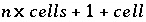, where cells is number of mobile cells and . Each immobile cell that is used must have a defined solution ( SOLUTION, SOLUTION_SPREAD, or SAVE data block) and either a MIX data block must be defined or, for the first-order exchange model, the exchange_factor must be defined (only applicable if stagnant_cells equals 1). Mixing will be performed at each diffusion/dispersion time step. EQUILIBRIUM_PHASES, EXCHANGE, GAS_PHASE, KINETICS, REACTION, REACTION_TEMPERATURE, SOLID_SOLUTIONS, and SURFACE may be defined for an immobile cell. Thermal diffusion in excess of hydrodynamic diffusion can only be calculated for the first-order exchange model. Optionally, stagnant or -st[ agnant].

stagnant_cells --Number of stagnant (immobile) cells associated with each mobile cell. Default is 0.

exchange_factor --Factor describing exchange between mobile and immobile cells (s^-1 ). The exchange_factor is used only if stagnant_cells is 1 and all immobile cells have the same properties. WARNING: If exchange_factor is entered, all previously defined MIX structures will be deleted and MIX structures for the first order exchange model for a dual porosity medium will be created. Default is 0.

--Porosity in each mobile cell. The is used only if stagnant_cells is 1 and all immobile cells have the same properties. Default is 0.

--Porosity in each immobile cell. The is used only if stagnant_cells is 1 and all immobile cells have the same properties. Default is 0.

Line 11: -thermal_diffusion temperature retardation factor, thermal diffusion coefficient

-thermal_diffusion--Defines parameters for calculating the diffusive part of heat transport. Diffusive heat transport will be calculated as a separate process if the temperature in any of the solutions of the transport domain differs by more than 1°C, and when the thermal diffusion coefficient is larger than the effective (aqueous) diffusion coefficient . Otherwise, diffusive heat transport is calculated as a part of aqueous diffusion. The temperature retardation factor is defined as the ratio of the heat capacity of the total aquifer over the heat capacity of water in the pores, and equals 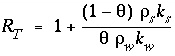, where is the water filled porosity, is density (kg/m³ ), k is specific heat (kJ°C^-1 kg^-1 ), and subscripts w and s indicate water and solid, respectively. The thermal diffusion coefficient can be estimated using , where is the heat conductivity of the aquifer, including pore water and solid (kJ°C^-1 m^-1 s^-1 ). The value of may be 100-1500 times larger than the aqueous diffusion coefficient, or about 1e-6 m² /s. A temperature change during transport is reduced by the temperature retardation factor (-) to account for the heat capacity of the matrix. Optionally, -th[ermal_diffusion].

retardation factor --Temperature retardation factor, unitless. Default is 2.0.

thermal diffusion coefficient --Thermal diffusion coefficient. Default is the aqueous diffusion coefficient.

Line 12: -initial_time initial_time

-initial_time--Identifier to set the time at the beginning of a transport simulation. The identifier sets the initial value of the variable controlled by -time in the SELECTED_OUTPUT data block. Optionally, initial_time or -i[ nitial_time].

initial_time --Time (seconds) at the beginning of the transport simulation. Default is the cumulative time including all preceding ADVECTION simulations for which -time_step has been defined and all preceding TRANSPORT simulations.

Line 13: -print_cells list of cell numbers

-print_cells--Identifier to select cells for which results will be written to the output file. Optionally, print, print_cells, or -pr[ int_cells]. Note the hyphen is required to avoid a conflict with the keyword PRINT.

list of cell numbers --Printing to the output file will occur only for these cell numbers. The list of cell numbers may be continued on the succeeding line(s). A range of cell numbers may be included in the list in the form m-n , where m and n are positive integers, m is less than n , and the two numbers are separated by a hyphen without intervening spaces. Default 1- cells .

Line 14: -print_frequency print_modulus

-print_frequency--Identifier to select shifts for which results will be written to the output file. Optionally, print_frequency, -print_f[ requency], output_frequency, or -o[ utput_frequency].

print_modulus --Printing to the output file will occur after every print_modulus advection shifts or diffusion periods. Default is 1.

Line 15: -punch_cells list of cell numbers

-punch_cells--Identifier to select cells for which results will be written to the selected-output file. Optionally, punch, punch_cells, -pu[ nch_cells], selected_cells, or -selected_c[ ells].

list of cell numbers --Printing to the selected-output file will occur only for these cell numbers. The list of cell numbers may be continued on the succeeding line(s). A range of cell numbers may be included in the list in the form m-n , where m and n are positive integers, m is less than n , and the two numbers are separated by a hyphen without intervening spaces. Default 1- cells .

Line 16: -punch_frequency punch_modulus

-punch_frequency--Identifier to select shifts for which results will be written to the selected-output file. Optionally, punch_frequency, -punch_f[ requency], selected_output_frequency, -selected_o[ utput_frequency].

punch_modulus --Printing to the selected-output file will occur after every punch_modulus advection shifts or diffusion periods. Default is 1.

Line 17: -dump dump file

-dump--Identifier to write complete state of a advective-dispersive transport simulation after every dump_modulus advection shifts or diffusion periods. The file is formatted as an input file that can be used to restart calculations. Optionally, dump or -du[ mp].

dump file --Name of file to which complete state of advective-dispersive transport simulation will be written. Default is phreeqc.dmp .

Line 18: -dump_frequency dump_modulus

-dump_frequency--Complete state of a advective-dispersive transport simulation will be written to dump file after dump_modulus advection shifts or diffusion periods. Optionally, dump_frequency or -dump_f[ requency].

dump_modulus --Complete state will be printed after dump_modulus advection shifts or diffusion periods. Default is shifts /2 or 1, whichever is larger.

Line 19: -dump_restart shift number

-dump_restart--If an advective-dispersive transport simulation is restarted from a dump file, the starting shift number is given on this line. Optionally, dump_restart or -dump_r[ estart].

shift number --Starting shift number for the calculations, if restarting from a dump file. The shift number is written in the dump file by PHREEQC. It equals the shift number at which the dump file was created. Default is 1.

Line 20: -warnings [( True or False )]

-warnings--Identifier enables or disables printing of warning messages for transport calculations. In some cases, transport calculations could produce many warnings that are not errors. Once it is determined that the warnings are not due to erroneous input, disabling the warning messages can avoid generating large output files. Optionally, warnings, warning, or -w[ arnings].

[( True or False )]--If value is true, warning messages are printed to the screen and the output file; if value is false, warning messages are not printed to the screen or the output file. The value set with -warnings is retained in all subsequent transport simulations until changed. Default is True, value at beginning of run is True.

Notes

The advective-dispersive transport capabilities of PHREEQC are derived from a formulation of 1D, advective-dispersive transport presented by Appelo and Postma (1993). The 1D column is defined by a series of cells (number of cells is cells ), each of which has the same pore volume. Lengths are defined for each cell and the time step ( time step ) gives the time necessary for a pore volume of water to move through each cell. Thus, the velocity of water in each cell is determined by the length of the cell divided by the time step. In the example data block, a column of five cells ( cells ) is modeled and 5 pore volumes of filling solution are moved through the column ( shifts / cells is 5). The total time of the simulation is 25 years ( ). The total length of the column is 6 m (four 1-m cells and one 2-m cell).

At each shift, advection is simulated by moving solution cells-1 to cell cells , solution cells-2 to cell cells-1 , and so on, until solution 0 is moved to cell 1 (upwind scheme). With flux-type boundary conditions, the dispersion steps follow the advective shift. With Dirichlet boundary conditions, the dispersion step and the advective shift are alternated. After each advective shift and dispersion step, kinetic reactions and chemical equilibria are calculated. The moles of pure phases and the compositions of the exchange assemblage, surface assemblage, gas phase, solid-solution assemblage, and kinetic reactants in each cell are updated after each chemical equilibration.

The -time_step identifier defines the length of time associated with each advective shift or diffusion period. This time step may be subdivided into smaller dispersion time steps if necessary to calculate dispersion accurately. Each dispersion time step may be further subdivided to integrate the kinetic reactions ( KINETICS data block). Kinetic reactions are likely to slow the calculations by up to a factor of six or more compared to pure equilibrium calculations.

The numerical scheme is for cell-centered concentrations, which has consequences for data interpretation. Thus, the composition in a boundary cell is a half-cell distance away from the column outlet and needs a half time step to arrive at (or from) the column end. The half time step must be added to the total residence time in the column when effluent from a column is simulated [use (TOTAL_TIME + time step /2) for time, see example 15, or (STEP_NO + 0.5)/ cells ) for pore volumes, see example 11]. The kinetics time for advective transport into the boundary cell is the advective time step divided by 2. Also, the cell-centered scheme does not account for dispersion in the border half-cell in case of a flux boundary condition. The identifier -correct_disp provides an option to correct the ignored dispersion, by increasing the dispersivity for all cells in the column by the appropriate amount. The correction will improve the comparison with analytical solutions for conservative elements when the number of cells is small.

It has been shown in the section "Transport in Dual Porosity Media" that a "dual porosity" model, in which part of the porosity allows advective flow and part of the porosity is accessible only by diffusion, can be developed with a first-order exchange model and with finite-differences, and both approaches can be defined in terms of a mixing among cells. With the TRANSPORT data block, one column of mobile cells is used to represent the part of the flow system in which advection occurs, and then additional immobile cells connected to the mobile cells are used to represent the stagnant zone that is accessible only by diffusion. The stagnant zone can be defined to be parallel or perpendicular to the column of mobile cells or to be a combination of the two by proper definition of mixing factors in MIX data blocks. A shortcut is available for the classical formulation of a dual porosity medium with a first-order rate of exchange. In this case, -stagnant is used to define one stagnant cell for each mobile cell ( stagnant_cells = 1), an exchange factor ( exchange_factor ) for the exchange between immobile and mobile cells, and the porosities and for the mobile and immobile cells. WARNING: If this shortcut method is used to define the stagnant zone, then all previously defined MIX structures will be deleted and MIX structures for first order exchange in a dual porosity medium are set up.

Thermal diffusion can be modeled for a stagnant zone with first-order exchange between mobile and immobile cells. Thermal exchange is calculated after subtracting the part that is associated with hydrodynamic diffusion (see "Transport of Heat"). PHREEQC uses the value of the diffusion coefficient to find the correct heat exchange factor, and the value entered with identifier -diffusion_coefficient should be the same as has been used in equation 125 to calculate the exchange factor .

Most of the information for advective-dispersive transport calculations must be entered with other keyword data blocks. Advective-dispersive transport assumes that solutions with numbers 1 through cells have been defined using SOLUTION, SOLUTION_SPREAD, or SAVE data blocks. In addition the infilling solution must be defined. If -flow direction is forward, solution 0 is the infilling solution; if -flow_direction is backward, solution cells + 1 is the infilling solution, if -flow direction is diffusion_only, then infilling solutions at both column ends are optional. If stagnant zones are modeled, solution compositions for the stagnant-zone cells must be defined with SOLUTION, SOLUTION_SPREAD, or SAVE data blocks.

Pure-phase assemblages may be defined with EQUILIBRIUM_PHASES or SAVE, with the number of the assemblage corresponding to the cell number. Likewise, an exchange assemblage, a surface assemblage, a gas phase, and a solid-solution assemblage can be defined for each cell through EXCHANGE, SURFACE, GAS_PHASE, SOLID_SOLUTIONS, or SAVE keywords, with the identifying number corresponding to the cell number. Kinetically controlled reactions can be defined for each cell through the KINETICS data block. Note that ranges of numbers can be used to define multiple solutions, exchange assemblages, surface assemblages, gas phases, solid-solution assemblages, or kinetic reactions simultaneously and that SAVE allows definition of a range of numbers. Constant-rate reactions can be defined for mobile or immobile cells through REACTION data blocks, again with the identifying number of the REACTION data block corresponding to the cell number. REACTION_TEMPERATURE data blocks can be used to specify the initial temperatures of the cells in the transport simulation. Temperatures in the cells may change during the transport simulation depending on the temperature distribution and the temperature retardation factor defined by -temp_retardation_factor.

By default, the composition of the solution, pure-phase assemblage, exchange assemblage, surface assemblage, gas phase, solid-solution assemblage, and kinetic reactants are printed for each cell for each shift. Use of -print_cells and -print_frequency will limit the amount of data written to the output file. If -print_cells has been defined then only the specified cells will be written, otherwise, all cells will be written. The identifier -print_frequency will restrict writing to the output file to those shifts that are evenly divisible by print_modulus . In the example data block, results for cells 1, 2, 3, and 5 are written to the output file after each integer pore volume (5 shifts) has passed through the column. Data written to the output file can be further limited with the keyword PRINT (see -reset false).

If a SELECTED_OUTPUT data block has been defined (recommended), then selected data are written to the selected-output file. Use of -punch_cells and -punch_frequency in the TRANSPORT data block will limit the data that are written to the selected-output file. If -punch_cells has been defined then only the specified cells will be written, otherwise, all cells will be written. The identifier -punch_frequency will restrict writing to the selected-output file to those shifts that are evenly divisible by punch_modulus . In the example data block, results are written to the selected-output file for cells 2, 3, 4, and 5 after each integer pore volume (5 shifts) has passed through the column.

At the end of a advective-dispersive transport simulation, all the physical and chemical data (for example, compositions of solutions, equilibrium-phase assemblages, surfaces, exchangers, solid solutions, and kinetic reactants) are automatically saved and are identified by the cell number in which they reside. These data are available for subsequent simulations within a single run. Transient conditions can be simulated by including subsequent TRANSPORT data blocks, which may define new chemical boundary and transport conditions. Only parameters that differ from the previous advective-dispersive transport simulation need to be redefined, such as new infilling solution ( SOLUTION 0), a change from advection to diffusion only ( -flow_direction diffusion_only), or a change in flow direction from forward to backward ( -flow_direction backward). All parameters not specified in the new TRANSPORT data block remain the same as the previous advective-dispersive transport simulation. Normally, the diffusion coefficient, lengths of cells, dispersivities, and stagnant zone definitions would remain the same through all advective-dispersive transport simulations and thus need not be redefined.

For long advective-dispersive transport calculations, it may be desirable to save intermediate states in the calculation, either because of hardware failure or because of nonconvergence of the numerical method. The -dump_frequency identifier allows intermediate states to be saved at intervals during the calculation. The -dump identifier allows the definition of a file name in which to write these intermediate states. The dump file is formatted as an input file for PHREEQC, so calculations can be resumed from the point at which the dump file was made. The -dump_restart identifier allows a shift number to be specified from which to restart the calculations.

TRANSPORT

Example data block

Explanation

Notes

Example problems

Related keywords