EXAMPLES
The conceptual model for the calculation of this example assumes that brines initially filled the aquifer. The aquifer contains calcite, dolomite, clays with cation exchange capacity, and hydrous ferric oxide surfaces, and initially, the cation exchanger and surfaces are in equilibrium with the brine. The aquifer is assumed to be recharged with rain water that is concentrated by evaporation and equilibrates with calcite and dolomite in the vadose zone. This water then enters the saturated zone and reacts with calcite and dolomite in the presence of the cation exchanger and hydrous ferric oxide surfaces.
The calculations use the advective transport capabilities of PHREEQC with just a single cell representing the saturated zone. A total of 200 pore volumes of recharge water are advected into the cell and, with each pore volume, the water is equilibrated with the minerals, cation exchanger, and the surfaces in the cell. The evolution of water chemistry in the cell represents the evolution of the water chemistry at a point within the saturated zone of the aquifer.
The amount of arsenic on the surface was estimated from sequential extraction data on core samples (Mosier and others, 1991). Arsenic concentrations in the solid phases generally ranged from 10 to 20 ppm., which corresponds to 1.3 to 2.6 mmol/L arsenic. The number of surface sites were estimated from the amount of extractable iron in sediments, which ranged from 1.6 to 4.4 percent (Mosier and others, 1991). A content of 2 percent iron for the sediments corresponds to 3.4 mol/L of iron. However, most of the iron is in goethite and hematite, which have far fewer surface sites than hydrous ferric oxides. The fraction of iron in hydrous ferric oxides was arbitrarily assumed to be 0.1. Thus, a total of 0.34 mol of iron was assumed to be in hydrous ferric oxides, and using a value of 0.2 for the number of sites per mole of iron, a total of 0.7 mol of sites per liter was used in the calculations. A gram formula weight of 89 was used to estimate that the mass of hydrous ferric oxides was 30 g/L. The specific surface area was assumed to be 600 m2/g.
TITLE Example 10.--Transport with equilibrium_phases,
   exchange, and surface reactions
SOLUTION 1 Brine
        pH      5.713
        pe      4.0     O2(g)   -0.7
        temp    25.
        units   mol/kgw
        Ca      .4655
        Mg      .1609
        Na      5.402
        Cl      6.642           charge
        C       .00396
        S       .004725
        As      .05 umol/kgw
EQUILIBRIUM_PHASES 1
        Dolomite        0.0     1.6
        Calcite         0.0     0.1
EXCHANGE 1
        -equil with solution 1
        X       1.0
SURFACE 1
        -equil solution 1
# assumes 1/10 of iron is HFO
        Hfo_w           0.07    600.    30.
END
SOLUTION 0 20 x precipitation
        pH      4.6
        pe      4.0     O2(g)   -0.7
        temp    25.
        units   mmol/kgw
        Ca      .191625
        Mg      .035797
        Na      .122668
        Cl      .133704
        C       .01096
        S       .235153         charge
EQUILIBRIUM_PHASES 0
        Dolomite        0.0     1.6
        Calcite         0.0     0.1
        CO2(g)          -1.5    10.
SAVE solution 0
END
SURFACE_SPECIES
        Hfo_wOH + Mg+2 = Hfo_wOMg+ + H+
#       log_k -4.6
        log_k -15.
        Hfo_wOH + Ca+2 = Hfo_wOCa+ + H+
#       log_k -5.85
        log_k -15.
TRANSPORT
        -cells 1
        -shifts 200
SELECTED_OUTPUT
        -file ex10.pun
        -totals Ca Mg Na Cl C S As
END
The brine that initially fills the aquifer was taken from Parkhurst, Christenson, and Breit (1993) and is given as solution 1 in the input data set for this example (table 18). The pure-phase assemblage containing calcite and dolomite is defined with the EQUILIBRIUM_PHASES 1 keyword. The number of cation exchange sites is defined with EXCHANGE 1 keyword and the number of surface sites are defined with SURFACE 1 keyword. Both the initial exchange and the initial surface composition are determined by equilibrium with the brine. The concentration of arsenic in the brine was determined by trial and error to give a total of approximately 2 mmol arsenic on the surface complexer, which is consistent with the sequential extraction data. The default data base, wateq4f.dat, was used for all thermodynamic data, with the exception of two surface reactions. After initial runs it was determined that much better results were obtained for arsenic concentrations if the calcium and magnesium surface complexation reactions were removed. The SURFACE_SPECIES data block was used to decrease the equilibrium constant for each of these two reactions by about 10 orders of magnitude. This effectively eliminated surface complexation reactions for calcium and magnesium. (Alternatively, these reactions could be removed from the default data base.) This is justified if cations and anions do not actually compete for the same sites. of 10-1.5. The second simulation in the input set generates this water composition and stores it as solution 0 (table 18).
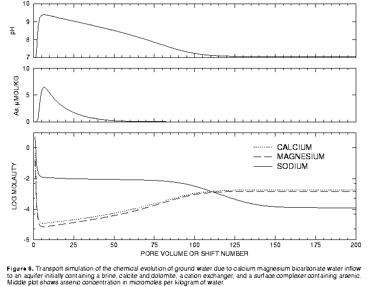
The results of the calculations are plotted on figure 6. During the initial 5 pore volumes, the large concentrations of sodium, calcium, and magnesium decrease such that sodium is the dominant cation and calcium and magnesium concentrations are small. The pH increases to more than 9.0 and arsenic concentrations increase to more than 5 mmol/kg water. Over the next 45 pore volumes the pH gradually decreases and the arsenic concentrations decrease to negligible concentrations. At about 100 pore volumes, the calcium and magnesium become the dominant cations and the pH stabilizes at the pH of the infilling recharge water.
The transport calculations produce three types of water in the aquifer, the initial brine, a sodium bicarbonate water, and a calcium and magnesium bicarbonate water, which are similar to the observed water types in the aquifer. The pH values are also consistent with the observations, although the peak near pH 9.5 is slightly too high. Sensitivity calculations indicate that the maximum pH depends on the amount of exchanger present. Decreasing the number of cation exchange sites decreases the maximum pH. Arsenic concentrations are also higher than the maximum values observed in the aquifer, which are in the range of 1 to 2 mmol/kg water. Lower maximum pH values would produce lower maximum arsenic concentrations. The stability constant for the surface complexation reactions have been taken directly from the literature; a minor decrease in the log K for the predominant arsenic complexation reaction would tend to decrease the maximum arsenic concentration as well. In conclusion, the model results, which were based largely on measured values and literature thermodynamic data provide a satisfactory explanation of the variation in major ion chemistry, pH, and arsenic concentrations within the aquifer.