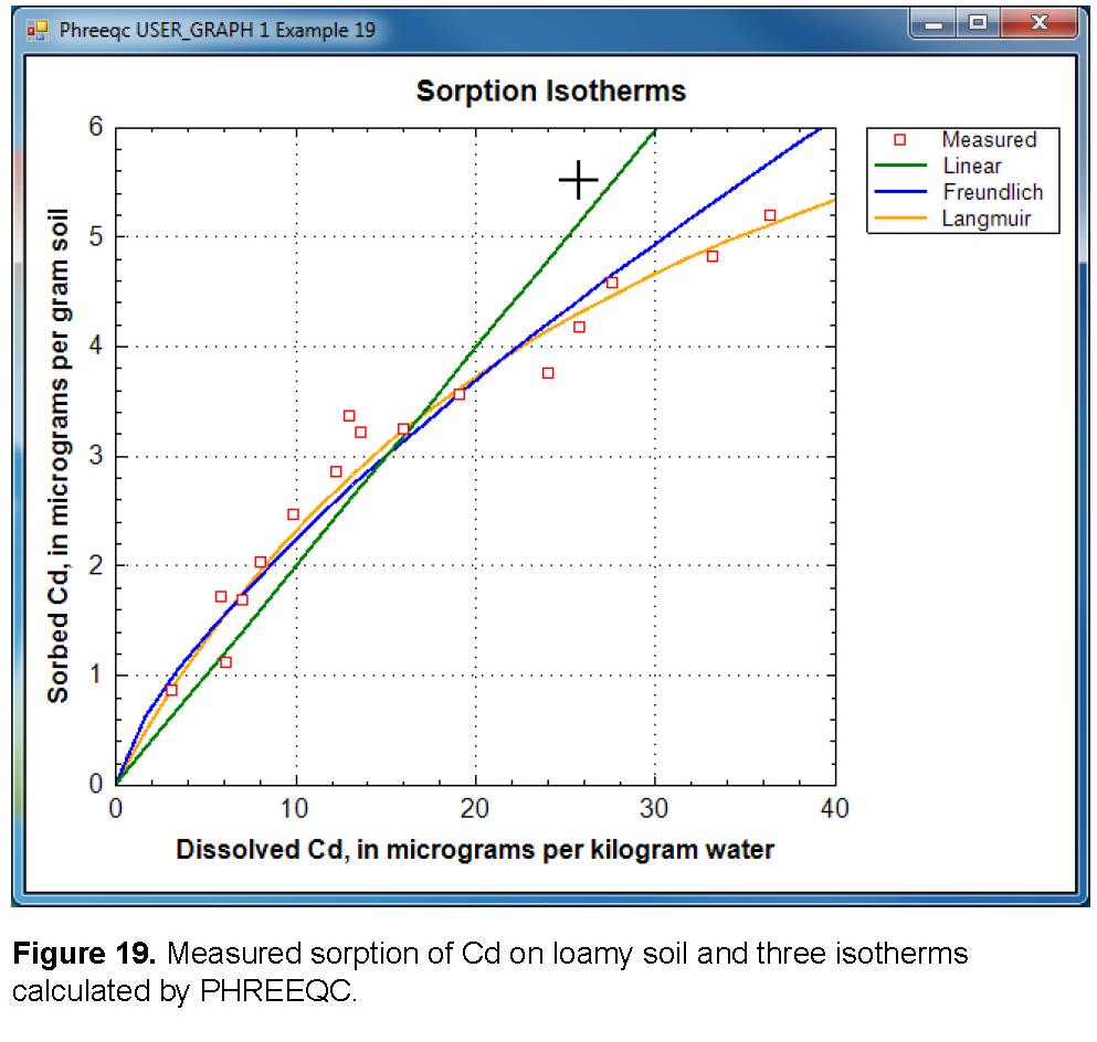
Sorption of heavy metals and organic pollutants on natural materials can be described by linear, Freundlich, or Langmuir isotherms. All three isotherms can be calculated by PHREEQC, as shown in this example for Cd+2 sorbing on a loamy soil (Christensen, 1984; Appelo and Postma, 2005). A more mechanistic approach, also illustrated here, is to model the distribution of Cd+2 over the sorbing components in the soil, in this case, in and on organic matter, clay minerals, and iron oxyhydroxides.
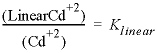
Figure 19 shows the measured sorbed concentration (μg/g soil, microgram per gram) as a function of solute concentration (μg/L water, microgram per liter), and three isotherms defined by:
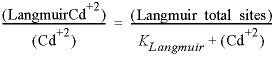 , (35)
where the brackets indicate concentrations in μg/g soil and μg/L water, and Linear, Freundlich, and Langmuir refer to the sorption sites that will be used in definitions for the SURFACE keyword.
The three isotherms correspond to reactions and mass-action equations that can be entered in PHREEQC as follows:
 , (38)
where the square brackets indicate activities (unitless).
The Langmuir isotherm (equation 35) and its PHREEQC formulation (equation 38) are equivalent for sorption of Cd on 1 g soil when (Langmuir_total_sites) / 112.4×10 6 = molesLangmuir sites, PHREEQC, and (KLangmuir / 112.4×10 6 )-1 = KLangmuir, PHREEQC, where 112.4×10 6 μg/mol (microgram per mole) is the atomic weight of Cd. Thus, the Langmuir isotherm represents a valid chemical reaction that can be defined in PHREEQC. That is not the case for the linear and the Freundlich isotherms because the equations do not account for the decrease of the “free” sites when Cd+2 sorbs. However, in PHREEQC the number of sorption sites can be made large; for example moleslinear, PHREEQC = 10100 mol, so that a decrease of a few moles of free sites by surface complexation will be negligible relative to the total number of free sites. In activity terms, the effect of the large number of sites is that [Linear] = 1 at all times in equation 36. By reducing the constant in the mass-action equation by the same large number, the required distribution is satisfied. Thus, Klinear, PHREEQC = Klinear / moleslinear, PHREEQC. Similarly for the Freundlich equation, KFreundlich, PHREEQC = KFreundlich / molesFreundlich, PHREEQC. The remaining problem with the Freundlich equation (equation 37) is that the stoichiometric coefficient for Cd+2 is n on the left-hand side of the equation, but is 1 on the right-hand side of the equation. This inconsistency can be ignored in PHREEQC by adding -no_check to the reaction equation.
The coefficients in the linear, Freundlich, and Langmuir isotherm equations that fit the measurements are taken from Appelo and Postma (2005). For the linear isotherm Klinear = 0.2 (L water / g soil), and for the Freundlich and Langmuir isotherms:
The input file (table 55) defines the sorption reactions with keywords SURFACE_MASTER_SPECIES and SURFACE_SPECIES. To avoid accumulation of charge in the solution, the sorption formula is specified to be surfaceCdCl2 with -mole_balance for each of the reactions, where surface is Linear, Freundlich, or Langmuir. The keyword SURFACE defines the moles of sites, and the identifier -no_edl specifies that the calculations will be done without the charge/potential term in the mass-action equations for the sorbed species. Next a 1 mM (millimolar) CaCl2 is entered with keyword SOLUTION, followed by a reaction of 0.7 mmol CdCl 2 in 20 steps (REACTION data block). USER_GRAPH plots the isotherms, and the experimental data are added to the plot with -plot_tsv_file ex19_meas.tsv.
Christensen (1984) measured the exchange capacity of the soil (CEC = 56 meq/kg, milliequivalent per kilogram), the iron-oxyhydroxide content (2,790 ppm Fe), and organic matter content (OM = 0.7 weight percent), which can be inserted in a deterministic PHREEQC model. The database phreeqc.dat contains the exchange reaction of Cd+2 and Ca+2 (the predominant cation in the experiment) with the exchange site X-, and the surface complexation reactions of Cd+2 on hydrous ferric oxide (Hfo). Christensen measured the iron content by extracting the soil with dithionite, which reduces and dissolves all amorphous and crystalline iron oxyhydroxides. It is assumed that only 10 percent of analyzed iron has the reactivity represented by Hfo in the phreeqc.dat database. The measured exchange capacity is entered as moles X-, although part of the exchange capacity is located in organic matter, which is modeled separately. Organic matter binds Cd+2 more strongly than clay minerals, so the overestimation of the clay exchange capacity is assumed to be negligible. However, the assumption is checked (and corrected) in the model results, from which the contribution of organic matter to the CEC is estimated by summing the Ca-complexes on humic acid and the calcium excess in the double layer.
Complexation on organic matter can be modeled with WHAM, the Windermere Humic Acid Model of Tipping and Hurley (Tipping and Hurley, 1992; Tipping, 1998; Lofts and Tipping, 2000). The WHAM model was designed for humic and fulvic acids in surface water, but it has been applied to Cd sorption on organic matter in soils (Shi and others, 2007). Complexation constants are defined for protons and cations on a number of monodentate and bidentate binding sites, which can be entered simply as SURFACE_SPECIES in PHREEQC. Furthermore, an empirical parameter for the charge-potential relation of the (probably spherical) humic molecules is incorporated into the Gouy Chapman relation that is used in PHREEQC by adjusting the specific surface area with a function that depends on the ionic strength of the solution (Appelo and Postma, 2005).
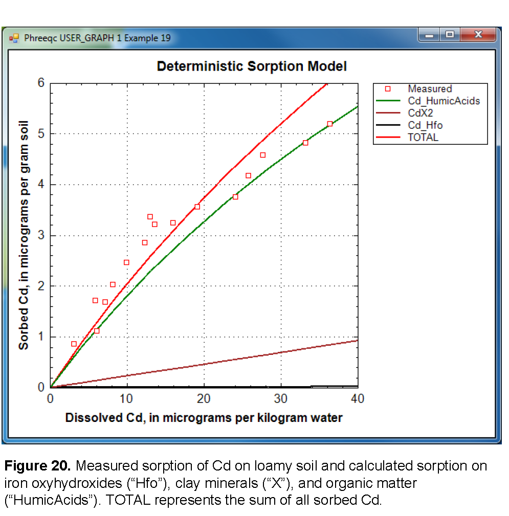
The input file (table 56) starts with the SOLUTION_MASTER_SPECIES for the complexing sites on humic acid and the SURFACE_SPECIES for protons, Cd+2 and Ca+2. Next the SURFACE is defined, with number of sites for 3.5 mg humic acid (1 g soil with 0.7 percent OM, is about 3.5 mg organic carbon, taken all as humic acid initially, but corrected to an active fraction by comparing model and measured results). In the WHAM model, the humic acid has a total charge of -7.1 meq/g (milliequivalent per gram), distributed over four monoprotic carboxylic sites (nHA carrying a charge of -2.84 meq/g humic acid), four monoprotic phenolic sites (nHB, charge = -1.42 meq/g humic acid) and twelve diprotic sites that combine carboxylic and phenolic charges (charge = -2.84 meq/g humic acid). Hfo, assumed to represent 10 percent of analyzed iron, is part of the same SURFACE. Keyword EXCHANGE defines the moles of X- in 1 g soil, the SOLUTION is 1 mM CaCl2 with a very small Cd+2 concentration to avoid a zero division in USER_GRAPH. USER_GRAPH prints the contribution of organic matter to the CEC and the distribution coefficient for Cd+2 (L/kg, liter per kilogram), and plots the sorption of Cd+2 by organic matter, clay exchange, and iron oxyhydroxides (fig. 20).
In line with many experimental results, figure 20 illustrates that Cd in soils is mainly bound to organic matter. The contribution of clay exchange is about 20 percent, and the contribution of iron-oxyhydroxide surface complexation is negligible. Actually, the sorbed concentration of Cd+2 on 3.5 mg humic acids would be nine times higher, but the concentration was reduced by multiplying with an active fraction of organic matter to match the measured data. The smaller active fraction is understandable because a soil contains lignin and a variety of other, less reactive compounds than the pure humic acid that formed the basis for the Tipping and Hurley database. Shi and others (2007) found an average active fraction of 0.6 for organic carbon concentrations that ranged from 0.18 to 7.15 weight percent in New Jersey soils, whereas Weng and others (2002) and Bonten and others (2008) used an active fraction of 0.3 for soil organic matter in the NICA-Donnan model.
Earlier it was assumed that the organic-matter contribution to the CEC was negligible. The assumption is checked by calculating the Ca exchanged on organic matter relative to the amount exchanged on clays. The amount of calcium exchanged on organic matter is printed in the output file for the largest cadmium concentration as:
Total Ca in/on organic matter = 1.1810e-006 CEC on OM = 4.2407e+000 %.
Although the correction is so small as to be unnecessary, the CEC attributed to clays should be reduced by a factor of 0.96 to account for the 4 percent of the exchange capacity that is located in or on organic matter.
 , (33)
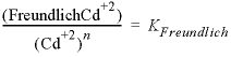 , and (34)
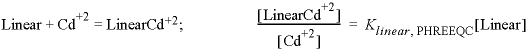 , (36)
 , (37)
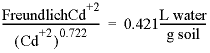 , and (39)
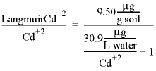 . (40)