Example 6.-- Reaction-Path Calculations

EXAMPLES

Example 6.-- Reaction-Path Calculations

In this example, the precipitation of phases as a result of incongruent dissolution of microcline (potassium feldspar) is investigated. Only a limited set of phases, microcline, gibbsite, kaolinite, and muscovite (potassium mica), is considered in this example. The reaction path for this set of phases was originally addressed by Helgeson and others (1969). In this example, the thermodynamic data for the phases (table 13, PHASES keyword) are derived from Robie and others (1978) and are the same as test problem 5 in the PHREEQE manual (Parkhurst and others, 1980).

Table 13. Input data set for example 6

TITLE Example 6A.--React to phase boundaries.
SOLUTION 1  PURE WATER
            pH    7.0 charge
          temp   25.0
PHASES 1
        Gibbsite
                Al(OH)3 + 3 H+ = Al+3 + 3 H2O
                log_k          8.049
                delta_h        -22.792 kcal
        Kaolinite
                Al2Si2O5(OH)4 + 6 H+ = H2O + 2 H4SiO4 + 2 Al+3
                log_k          5.708
                delta_h        -35.306 kcal
        Muscovite
                KAl3Si3O10(OH)2 + 10 H+ = 3 Al+3 + 3 H4SiO4 + K+
                log_k          12.970
                delta_h        -59.377 kcal
        Microcline
                KAlSi3O8 + 4 H2O + 4 H+ = Al+3 + 3 H4SiO4 + K+
                log_k          0.875
                delta_h        -12.467 kcal
END
TITLE Example 6A1.--Find amount of k-spar dissolved to 
                    reach gibbsite saturation.
SELECTED_OUTPUT
        -file           ex6.pun
        -activities     K+ H+ H4SiO4
        -si             Gibbsite Kaolinite Muscovite Microcline
        -equilibrium    Gibbsite Kaolinite Muscovite Microcline
USE solution 1
EQUILIBRIUM_PHASES 1
        Gibbsite        0.0     KAlSi3O8        10.0
        Kaolinite       0.0     0.0
        Muscovite       0.0     0.0
        Microcline      0.0     0.0
END
TITLE Example 6A2.--Find amount of k-spar dissolved to 
                    reach kaolinite saturation.
USE solution 1
EQUILIBRIUM_PHASES 1
        Gibbsite        0.0     0.0
        Kaolinite       0.0     KAlSi3O8        10.0
        Muscovite       0.0     0.0
        Microcline      0.0     0.0
END
TITLE Example 6A3.--Find amount of k-spar dissolved to 
                    reach muscovite saturation.
USE solution 1
EQUILIBRIUM_PHASES 1
        Gibbsite        0.0     0.0
        Kaolinite       0.0     0.0
        Muscovite       0.0     KAlSi3O8        10.0
        Microcline      0.0     0.0
END
TITLE Example 6A4.--Find amount of k-spar dissolved to 
                    reach k-spar saturation.
USE solution 1
EQUILIBRIUM_PHASES 1
        Gibbsite        0.0     0.0
        Kaolinite       0.0     0.0
        Muscovite       0.0     0.0
        Microcline      0.0     10.0
END
TITLE 
Example 6A5.--Find point with kaolinite present, 
              but no gibbsite.
USE solution 1
EQUILIBRIUM_PHASES 1
        Gibbsite        0.0     KAlSi3O8        10.0
        Kaolinite       0.0     1.0
END
TITLE 
Example 6A6.--Find point with muscovite present, 
              but no kaolinite
USE solution 1
EQUILIBRIUM_PHASES 1
        Kaolinite       0.0     KAlSi3O8        10.0
        Muscovite       0.0     1.0
END
TITLE Example 6B.--Path between phase boundaries.
USE solution 1
EQUILIBRIUM_PHASES 1
        Kaolinite       0.0     0.0
        Gibbsite        0.0     0.0
        Muscovite       0.0     0.0
        Microcline      0.0     0.0
REACTION 1
        Microcline      1.0
        0.04 0.08 0.16 0.32 0.64 1.0 2.0 4.0 
        8.0 16.0 32.0 40.0 50.0 umol
END
USE solution 1
EQUILIBRIUM_PHASES 1
        Muscovite               0.0     10.0
        Kaolinite       0.0     10.0
        Gibbsite        0.0     10.0
END
USE solution 1
EQUILIBRIUM_PHASES 1
        Microcline      0.0     10.0
        Muscovite       0.0     10.0
        Kaolinite       0.0     10.0
END

PHREEQC can be used to solve this problem in two ways: (1) the individual intersections of the reaction path and the phase boundaries on a phase diagram can be calculated, or (2) the reaction path can be calculated incrementally. In the former approach, no knowledge of the amounts of reaction is needed, but a number of simulations are needed to find the appropriate phase-boundary intersections. In the latter approach, only one simulation is needed, but knowledge of the appropriate amounts of reaction is necessary. Both approaches will be demonstrated in this example. PHREEQC does not have all of the logic for a complete reaction-path program (for example Helgeson and others, 1970, Wolery, 1979, Wolery and others, 1990); in particular, no automatic step-size-adjusting algorithm is present to determine the appropriate amount of irreversible reactions to add at each point along the path and to avoid overstepping phase boundaries. However, the ability to calculate directly the phase boundary intersections provides an efficient way to outline reaction paths on phase diagrams. Also, in the incremental approach, PHREEQC automatically finds the stable phase assemblage at each step, so overstepping phase boundaries does not cause any phase-rule violations.

Conceptually, the example considers the reactions that would occur if microcline were placed in a beaker and allowed to react slowly. As microcline dissolves, other phases may begin to precipitate. In this example, it is assumed that only gibbsite, kaolinite, or muscovite can form, and that these phases will precipitate reversibly if they reach saturation. Thus, phases precipitated at the beginning of the reaction may redissolve as the reaction proceeds.

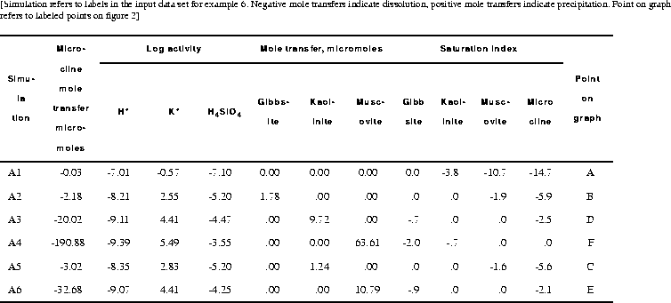
The input data set (table 13) first defines pure water with SOLUTION input and the thermodynamics of the phases with PHASES input. Some of the minerals are defined in the database file (phreeqc.dat), but inclusion in the input data set replaces any previous definitions for the duration of the run (the database file is not altered). In simulation A1, SELECTED_OUTPUT is used to produce a file of all the data that appear in table 14 and that were used to construct figure 2. SELECTED_OUTPUT specifies that the activities of potassium ion, hydrogen ion, and silicic acid; the saturation indices for gibbsite, kaolinite, muscovite, and microcline; and the total amounts in the phase assemblage and mole transfer for gibbsite, kaolinite, muscovite, and microcline will be written to the file ex6.pun after each calculation. The definitions for SELECTED_OUTPUT remain in effect for all simulations in the run, until a new SELECTED_OUTPUT data block is read, or until writing to the file is suspended with the identifier -selected_output in the PRINT keyword data block.

Table 14. Selected results for example 6

Simulation A1 allows microcline to react until equilibrium with gibbsite is reached. This is set up in EQUILIBRIUM_PHASES input by specifying equilibrium for gibbsite (saturation index equals 0.0) and an alternative reaction to reach equilibrium, KAlSi3O8 (the formula for microcline). A large amount microcline (10.0 mol) is present to assure equilibrium with gibbsite. Kaolinite, muscovite, and microcline are allowed to precipitate if they become saturated, but they can not dissolve because they were given zero initial moles in the phase assemblage. The amount of reaction that is calculated in this simulation is precisely enough to reach equilibrium with gibbsite, possibly including precipitation of one or more of the other minerals. No gibbsite will dissolve or precipitate. Simulations A2-A4 perform the same calculations for kaolinite, muscovite, and microcline.

Selected results for simulations A1-A4 are presented in table 14 and are plotted on figure 2 as points A, B, D, and F. The stability fields for the phases, which are based on the thermodynamic data, are outlined on the figure and are not calculated by the modeling in these simulations. From the positions of point B and D, it can be deduced that the reaction path should follow the gibbsite-kaolinite phase boundary to some intermediate point C before the path crosses the kaolinite field to point D. Similarly, there is a point E on the kaolinite-muscovite phase boundary, where the reaction path begins to cross the muscovite field to point F. Simulations A5 and A6 (table 13) solve for these two points. In simulation A5, point C is calculated by allowing microcline to dissolve to a point where kaolinite is at saturation and is present in the phase assemblage, while gibbsite is at saturation, but not present in the phase assemblage. Likewise, simulation A6 solves for the point where muscovite is at saturation and present in the phase assemblage, while kaolinite is at saturation, but is not present in the phase assemblage. Assigning an initial amount of 1 mol to kaolinite in A5 and muscovite in A6 is arbitrary; the amount must be sufficient to reach equilibrium with the mineral.

A simpler approach to determining the reaction path is simply to react microcline incrementally, allowing the stable phase assemblage among gibbsite, kaolinite, muscovite, and microcline to form at each point along the path. The only difficulty in this approach is to know the appropriate amounts of reaction to add. From points A and F in table 14, microcline dissolution ranges from 0.03 to 190.88 mmol. In part B (table 13) a logarithmic range of reaction increments is used to define the path (solid line) across the phase diagram from its beginning at gibbsite equilibrium (point A) to equilibrium with microcline (point F). However, the exact locations of points A through F will not be determined with the arbitrary set of reaction increments that are used in part B. The reaction path calculated by part B is plotted on the phase diagram in figure 2 with points A through F from part A included in the set of points.

Table 13. Input data set for example 6
Table 14. Selected results for example 6

User's Guide to PHREEQC - 07 MAY 96

[Next] [Previous] [Up] [Top]