First-Order Exchange Approximation
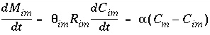
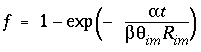
Diffusive exchange between mobile and immobile water can be formulated in terms of a mixing process between mobile and stagnant cells. In the following derivation, one stagnant cell is associated with one mobile cell. The first-order rate expression for diffusive exchange is
 , (119)
where subscript
m
indicates mobile and
im
indicates immobile,
M
im
are moles of chemical in the immobile zone,  is porosity of the stagnant (immobile) zone (a fraction of total volume, unitless),
R
im
is retardation in the stagnant zone (unitless),
C
im
is the concentration in stagnant water (mol/kgw),
t
is time (s),
C
m
is the concentration in mobile water (mol/kgw), and
is porosity of the stagnant (immobile) zone (a fraction of total volume, unitless),
R
im
is retardation in the stagnant zone (unitless),
C
im
is the concentration in stagnant water (mol/kgw),
t
is time (s),
C
m
is the concentration in mobile water (mol/kgw), and  is the exchange factor (s
-1
). The retardation is equal to
R
= 1 +
dq
/
dC,
which is calculated implicitly by PHREEQC through the geochemical reactions. The retardation contains the change
dq
in concentration of the chemical in the solid due to
all
chemical processes including exchange, surface complexation, kinetic and mineral reactions; it may be non-linear with solute concentration and it may vary over time for the same concentration.
is the exchange factor (s
-1
). The retardation is equal to
R
= 1 +
dq
/
dC,
which is calculated implicitly by PHREEQC through the geochemical reactions. The retardation contains the change
dq
in concentration of the chemical in the solid due to
all
chemical processes including exchange, surface complexation, kinetic and mineral reactions; it may be non-linear with solute concentration and it may vary over time for the same concentration.
The equation can be integrated with the following initial conditions:
 and
and  , at
t
= 0, and by using the mole-balance condition:
, at
t
= 0, and by using the mole-balance condition: 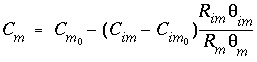 .
.
The integrated form of equation 119 is then:
 , (120)
where 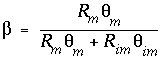 ,
,  ,
,  is the water filled porosity of the mobile part (a fraction of total volume, unitless), and
R
m
is the retardation in the mobile area.
is the water filled porosity of the mobile part (a fraction of total volume, unitless), and
R
m
is the retardation in the mobile area.
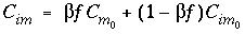
A mixing factor, mixf im , can be defined that is a constant for a given time t :
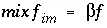 . (121)
When mixf im is entered in equation 120, the first-order exchange is shown to be a simple mixing process in which fractions of two solutions mix:
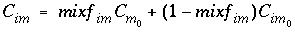 . (122)
Similarly, an equivalent mixing factor, mixf m , for the mobile zone concentrations is obtained with the mole-balance equation:
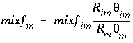 (123)
(123)and the concentration of C m at time t is
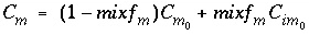 . (124)
The exchange factor  can be related to specific geometries of the stagnant zone (Van Genuchten, 1985). For example, when the geometry is spherical, the relation is
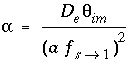 , (125)
where
D
e
is the diffusion coefficient in the sphere (m
2
/s),
a
is the radius of the sphere (m), and  is a shape factor for sphere-to-first-order-model conversion (unitless). Other geometries can likewise be transformed to a value for
  using other shape factors (Van Genuchten, 1985). These shape factors are given in table 1.
|
2 r o = outer diameter of pipe (Enter wall thickness r o - r i = a in Equation 125). |
|||


An analytical solution is known for a pulse input in a medium with first-order mass transfer between mobile and stagnant water (Van Genuchten, 1985; Toride and others, 1993); example 13 defines a simulation that can be compared with the analytical solution. A 2 m column is discretized in 20 cells of 0.1 m. The resident solution is 1 mM KNO 3 in both the mobile and the stagnant zone. An exchange complex of 1 mM is defined, and exchange coefficients are adapted to give linear retardation R = 2 for Na + . A pulse that lasts for 5 shifts of 1 mM NaCl is followed by 10 shifts of 1 mM KNO 3 . The Cl ( R = 1) and Na ( R = 2) profiles are calculated as a function of depth.
The transport variables are  = 0.3;
  = 0.1;
v
m
= 0.1 / 3600 = 2.778e-5 m/s; and
= 0.1;
v
m
= 0.1 / 3600 = 2.778e-5 m/s; and  = 0.015 m. The stagnant zone consists of spheres with radius a = 0.01 m, diffusion coefficient
D
e
= 3.e-10 m
2
/s, and a shape factor
= 0.015 m. The stagnant zone consists of spheres with radius a = 0.01 m, diffusion coefficient
D
e
= 3.e-10 m
2
/s, and a shape factor  = 0.21. This gives an exchange factor
  = 6.8e-6 s
-1
. In the PHREEQC input file
= 6.8e-6 s
-1
. In the PHREEQC input file  ,
,  , and
, and  must be given;
R
m
and
R
im
are calculated implicitly by PHREEQC through the geochemical reactions.
must be given;
R
m
and
R
im
are calculated implicitly by PHREEQC through the geochemical reactions.
Figure 4 shows the comparison of PHREEQC with the analytical solution (obtained with CXTFIT, version 2, Toride and others, 1995). The agreement is excellent for Cl
-
(
R
= 1), but the simulation shows numerical dispersion for Na
+
(
R
= 2). When the grid is made finer so that  is equal to or smaller than
  (0.015 m), numerical dispersion is much reduced. In the figure, the effect of a stagnant zone is to make the shape of the pulse asymmetrical. The leading edge is steeper than the trailing edge, where a slow release of chemical from the stagnant zone maintains higher concentrations for a longer period of time.
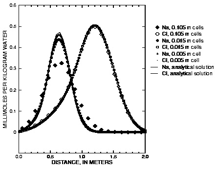
Figure 4. --Analytical solution for transport with stagnant zones, a pulse input, and ion-exchange reactions compared with PHREEQC calculations at various grid spacings.
 and
and  , transform to finite differences for an arbitrarily shaped cell
j
:
, transform to finite differences for an arbitrarily shaped cell
j
: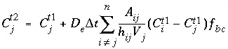 , (126)
 is the concentration in cell
j
at the current time,
is the concentration in cell
j
at the current time,  is the concentration in cell
j
after the time step,
is the concentration in cell
j
after the time step,  is the time step [s, equal to (
 )
D
in PHREEQC],
i
is an adjacent cell,
A
ij
is shared surface area of cell
i
and
j
(m
2
),
h
ij
is the distance between midpoints of cells
i
and
j
(m),
V
j
is the volume of cell
j
(m
3
), and
f
bc
is a factor for boundary cells (-). The summation is for all cells (up to
n
) adjacent to
j
. When
A
ij
and
h
ij
are equal for all cells, a central difference algorithm is obtained that has second-order accuracy [
O
(
h
)
2
]. It is therefore advantageous to make the grid regular.
)
D
in PHREEQC],
i
is an adjacent cell,
A
ij
is shared surface area of cell
i
and
j
(m
2
),
h
ij
is the distance between midpoints of cells
i
and
j
(m),
V
j
is the volume of cell
j
(m
3
), and
f
bc
is a factor for boundary cells (-). The summation is for all cells (up to
n
) adjacent to
j
. When
A
ij
and
h
ij
are equal for all cells, a central difference algorithm is obtained that has second-order accuracy [
O
(
h
)
2
]. It is therefore advantageous to make the grid regular. when
when  (or if the concentration is constant in the mobile region, Appelo and Postma, 1993, p. 376). Likewise,
f
bc
= 0 when
V
m
= 0. To a good approximation therefore,
(or if the concentration is constant in the mobile region, Appelo and Postma, 1993, p. 376). Likewise,
f
bc
= 0 when
V
m
= 0. To a good approximation therefore,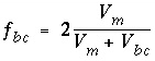 . (127)
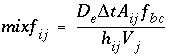 (128)
(128)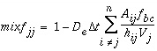 , (129)
 . (130)
 , which can be achieved by increasing the number of mobile cells. An example calculation is given in example